Introduction and overview
We’ll be using the OSGeo Live desktop to import some Ordnance Survey Open Roads data into a PostGIS database. Once loaded and configured the data will be built into a network topology for use with pgRouting. With a working network we’ll explore the different routing solutions in QGIS with the pgRoutingLayer plugin. If there is time at the end we’ll look at using PostgreSQL functions.
Step 0: Initial setup
For best results from this workshop the OSGeo Live environment needs to be installed in a VM or spun up as a live desktop session (off USB or DVD).
- Download either the VM image (4GB) for VirtualBox or the ISO (32bit (4GB) or 64bit (4GB)) for a USB drive.
- You can also set up your own instance of PostgreSQL, PostGIS, pgRouting, pgAdmin and QGIS but these instructions designed for use with the OSGeo Live environment.
Get the data: Nextcloud Link
Get VirtualBox here or VMWare Player here or, if you’re running Linux, your package manager.
To complete this workshop you will either need to boot your laptop from the live DVD or install one of the virtualisation applications and run the ISO or VMDK as a virtual machine. You’ll need to be able to access the internet and also your USB ports. If you could test this before the workshop it would help make the experience a good one for all.
Step 1: View the data in QGIS
Boot into OSGeo Live or start your virtual machine.
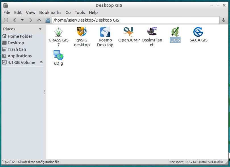
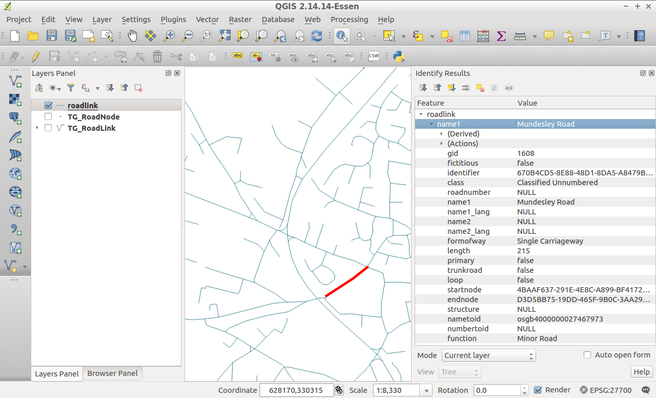
Open QGIS (Start > Geospatial > Desktop GIS > QGIS) or look in the Desktop GIS folder on the desktop. The version of QGIS available is 2.14 Essen which is not cutting edge but will work for this exercise.
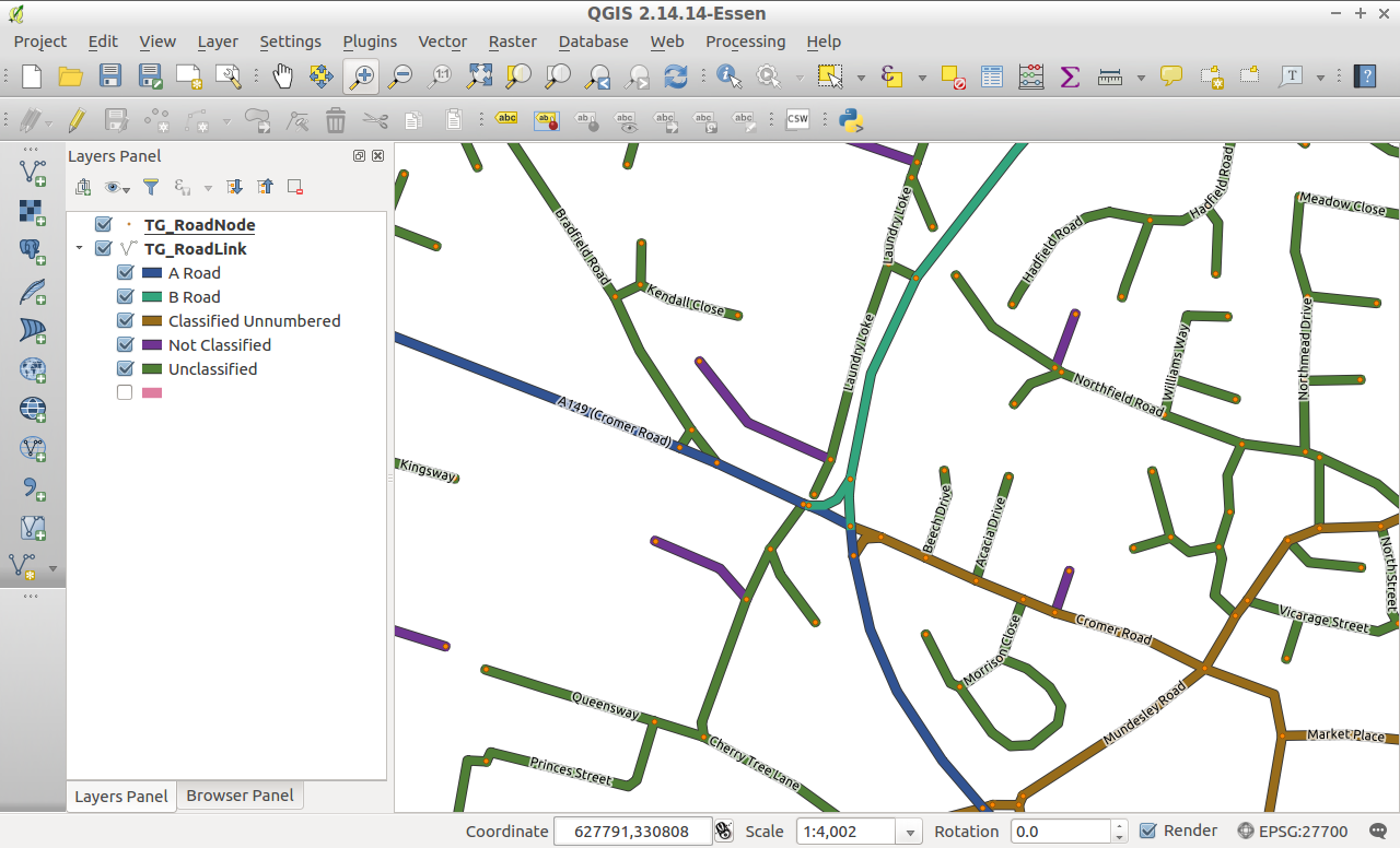
Browse to the data folder holding the roadlink and roadnode shapefiles you downloaded.
Drag the shapefiles onto the QGIS canvas. Use the identify tool or open the attribute table and node that Open Roads now uses UUID for road link IDs and also start and end nodes. During the load process we will create an INTEGER field to use with pgRouting as it can’t handle the UUID strings.
Step 2: Check the PostGIS database
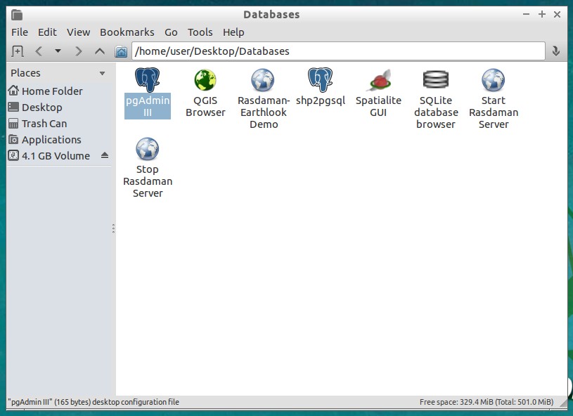
Open pgAdmin (Start > Geospatial > Databases > pgAdmin III) or look in the Databases folder on the desktop.
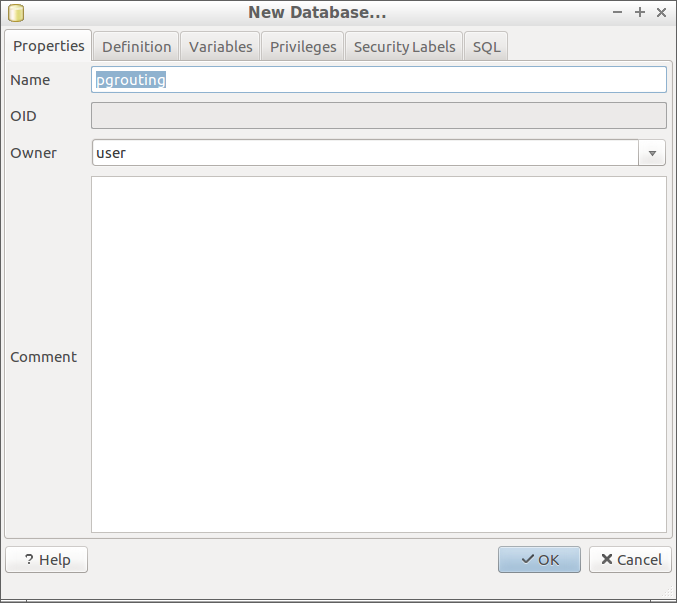
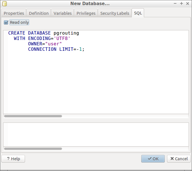
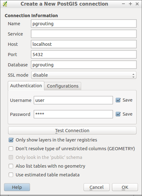
We will create a new database called pgrouting and install the postgis and pgrouting extensions. Connect to the local database server and expand the tree. Right click on Databases and choose New database. In the window that appears add the database name, pgrouting, and the owner, user, and click OK.
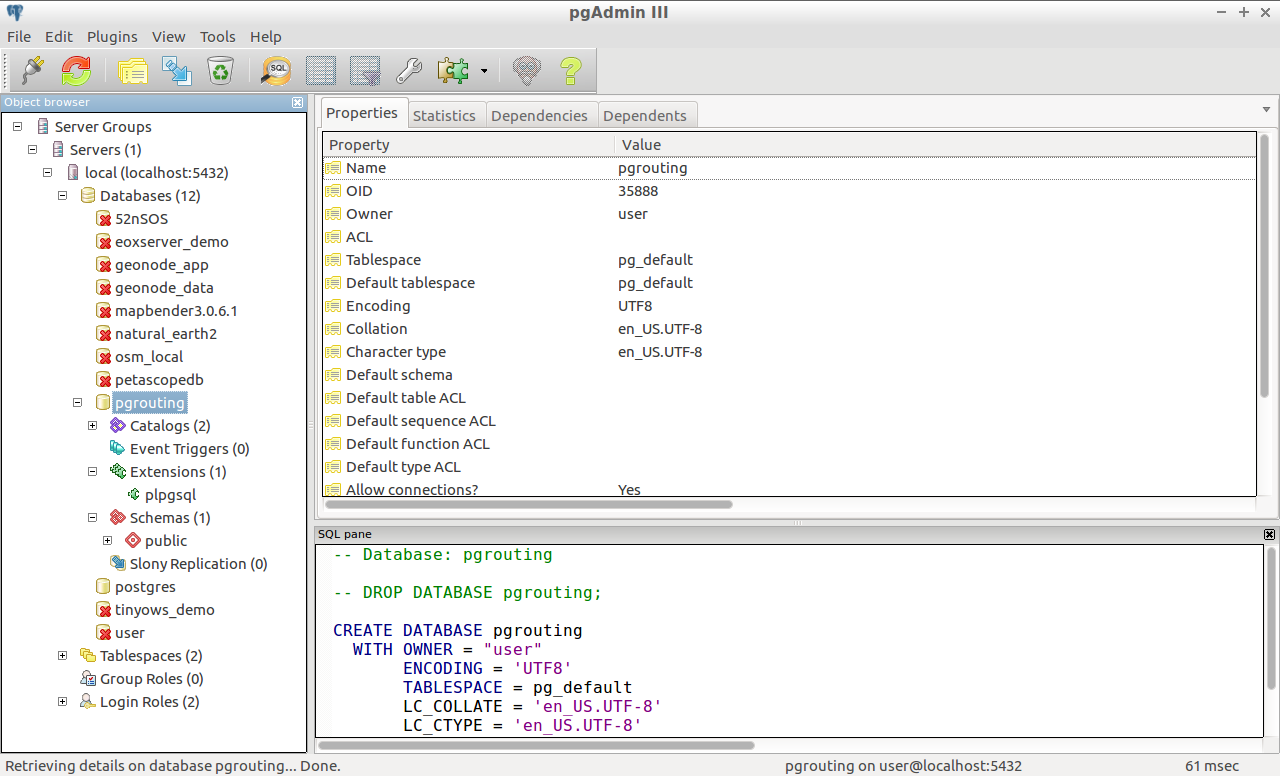
Refresh the database connection and see that pgrouting has been created.
Select the database to highlight it and open a query window. By selecting the database first, the query window know to execute any SQL against that database. Copy the following into the window:
CREATE EXTENSION postgis;
CREATE EXTENSION postgis_topology;
CREATE EXTENSION pgrouting;
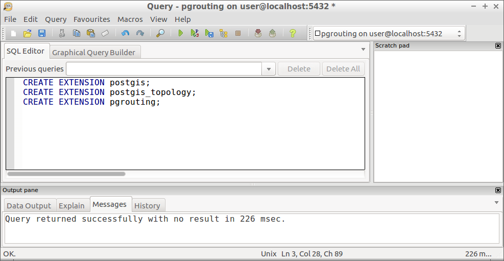
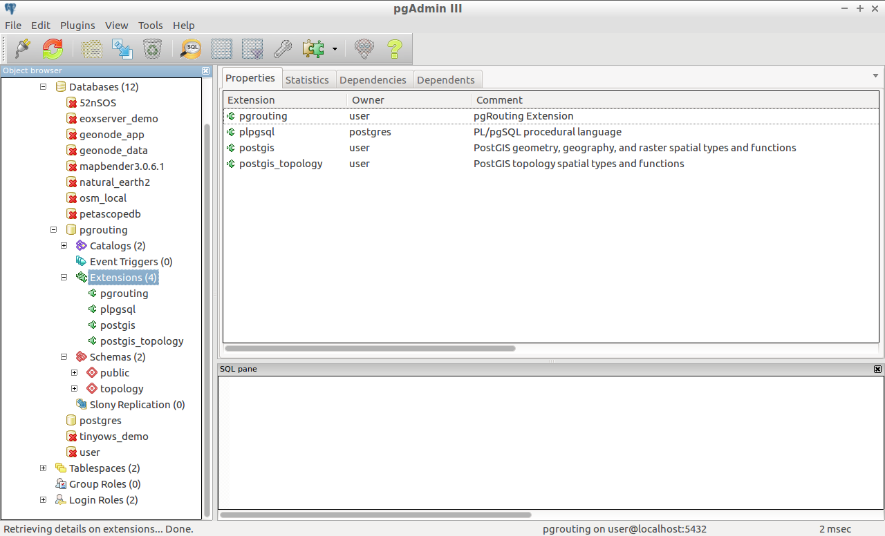
To execute each statement you can highlight the line and press F5. The message window will tell you whether it completed successfully or not. Close the window, ignoring any messages to save, and refresh the database connection. Look at the available extensions and see the new ones we have created. We now have a spatial database with routing capability. That wasnae so bad, was it?
Check connections: local (user / user)
Check database: pgrouting
Check schema: public
Check functions: pgr_* and st_*
Check extensions: pgRouting and PostGIS
Step 3: Load data from QGIS to PostGIS
Open or switch back to QGIS.
Create a new connection to our pgRouting database using the details above.
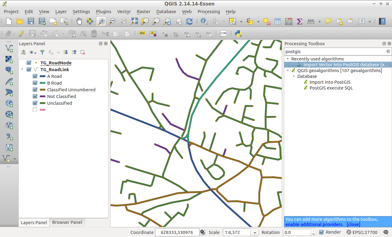
Open the Processing Toolbox (Processing > Toolbox) and search for PostGIS.
Pick and open the Import vector layer to PostGIS database (existing connection) tool from the results.
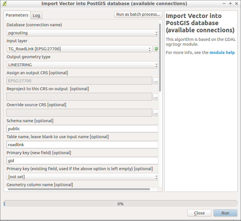
Set the following:
- Database connection name:
pgrouting - Input layer:
roadlink - Output geometry type:
linestring - Output CRS:
EPSG:27700 - Schema name:
public - Table name: leave blank to use existing name
- Primary key:
gid - Geometry column name:
geometry - Uncheck
Promote to Multipart(pgRouting likes LINESTRING and not MULTILINESTRING)
Note the OGR command in the box at the bottom - this could be copied into a batch file or shell script and reused.
The primary key field, gid, is important here as it is used when building the network topology and nodes later on.
Click the RUN button to load the shapefile into the database. Takes a few seconds.
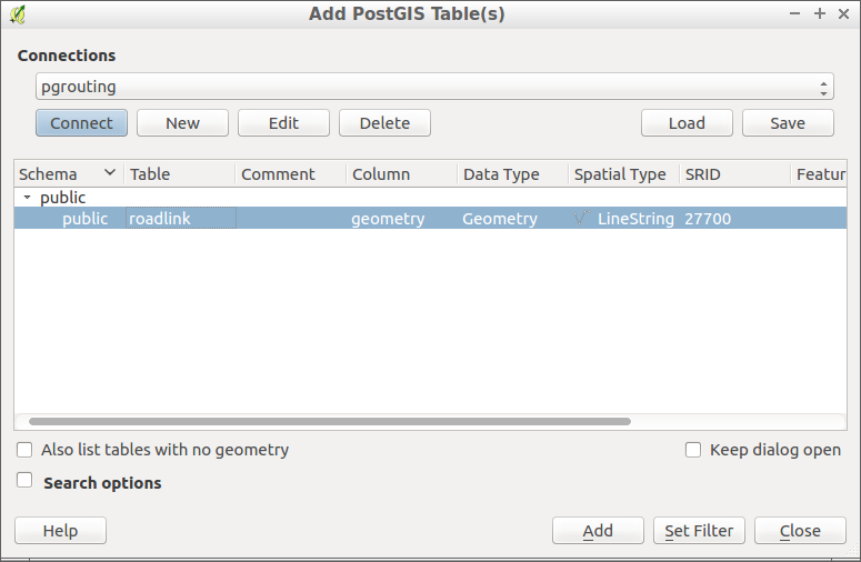
When the load has completed close the tool. Click the Add PostGIS layer button (blue elephant) and connect to the pgRouting database. Select the roadlink layer and click Add. Note that it is in EPSG:27700. The layer will be added to the QGIS canvas and will match the shapefile version already there. Use the identify tool to select a link and check the attributes.
Step 4: Add the pgRouting fields
Open or switch to PgAdminIII.
Navigate to the tables in the public schema of the pgRouting database. Click the SQL button on the top menu bar to open a SQL editor window. We’ll be using this to update our roadlink table with the fields and values that pgRouting needs.
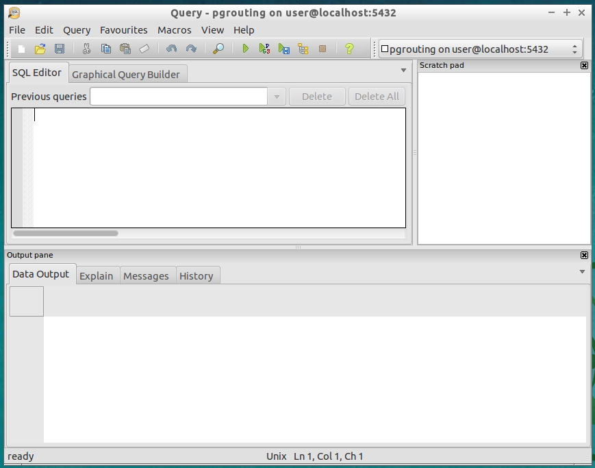
This section is a straightforward copy and paste exercise but we’ll go through it step by step.
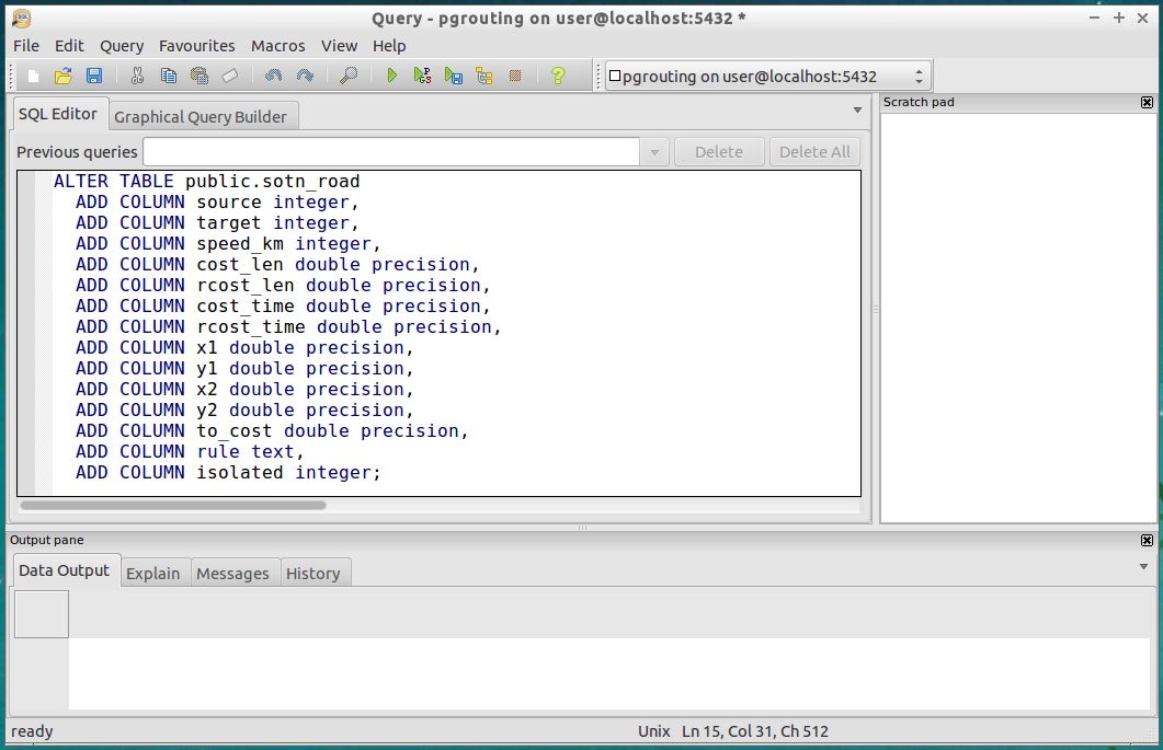
4.1 First, add the columns required to the roadlink table:
ALTER TABLE public.roadlink
  ADD COLUMN source integer,
  ADD COLUMN target integer,
  ADD COLUMN speed_km integer,
  ADD COLUMN cost_len double precision,
  ADD COLUMN rcost_len double precision,
  ADD COLUMN cost_time double precision,
  ADD COLUMN rcost_time double precision,
  ADD COLUMN x1 double precision,
  ADD COLUMN y1 double precision,
  ADD COLUMN x2 double precision,
  ADD COLUMN y2 double precision,
  ADD COLUMN to_cost double precision,
  ADD COLUMN rule text,
  ADD COLUMN isolated integer;
4.2 Create the required indices on the source and target fields for the fast finding of the start and end of the route. The source and target fields are populated with the node IDs that are created when the network topology is built later on.
CREATE INDEX roadlink_source_idx ON public.roadlink USING btree(source);
CREATE INDEX roadlink_target_idx ON public.roadlink USING btree(target);
4.3 Populate the line end coordinate fields (used in the Astar function).
UPDATE public.roadlink
  SET x1 = st_x(st_startpoint(geometry)),
    y1 = st_y(st_startpoint(geometry)),
    x2 = st_x(st_endpoint(geometry)),
    y2 = st_y(st_endpoint(geometry));
4.4 Use the length of the road link as the distance cost.
UPDATE public.roadlink
  SET cost_len = ST_Length(geometry),
  rcost_len = ST_Length(geometry);
4.5 Set the average speed depending on road class and the nature of the road using the class and formofway fields. Adjust the speeds here as you see fit. Note that I have used kilometres per hour and not miles per hour.
UPDATE public.roadlink SET speed_km =
  CASE
    WHEN class = 'A Road' AND formofway = 'Roundabout' THEN 20
    WHEN class = 'A Road' AND formofway = 'Collapsed Dual Carriageway' THEN 60
    WHEN class = 'A Road' AND formofway = 'Dual Carriageway' THEN 60
    WHEN class = 'A Road' AND formofway = 'Single Carriageway' THEN 55
    WHEN class = 'A Road' AND formofway = 'Slip Road' THEN 35
    WHEN class = 'A Road' AND formofway = 'Shared Use Carriageway' THEN 50
    WHEN class = 'B Road' AND formofway = 'Single Carriageway' THEN 50
    WHEN class = 'B Road' AND formofway = 'Collapsed Dual Carriageway' THEN 55
    WHEN class = 'B Road' AND formofway = 'Slip Road' THEN 35
    WHEN class = 'B Road' AND formofway = 'Roundabout' THEN 20
    WHEN class = 'B Road' AND formofway = 'Dual Carriageway' THEN 55
    WHEN class = 'B Road' AND formofway = 'Shared Use Carriageway' THEN 50
    WHEN class = 'Motorway' AND formofway = 'Collapsed Dual Carriageway' THEN 70
    WHEN class = 'Motorway' AND formofway = 'Dual Carriageway' THEN 70
    WHEN class = 'Motorway' AND formofway = 'Roundabout' THEN 20
    WHEN class = 'Motorway' AND formofway = 'Slip Road' THEN 35
    WHEN class = 'Motorway' AND formofway = 'Single Carriageway' THEN 60
    WHEN class = 'Motorway' AND formofway = 'Shared Use Carriageway' THEN 50
    WHEN class = 'Classified Unnumbered' AND formofway = 'Roundabout' THEN 20
    WHEN class = 'Classified Unnumbered' AND formofway = 'Single Carriageway' THEN 50
    WHEN class = 'Classified Unnumbered' AND formofway = 'Slip Road' THEN 35
    WHEN class = 'Classified Unnumbered' AND formofway = 'Dual Carriageway' THEN 55
    WHEN class = 'Classified Unnumbered' AND formofway = 'Collapsed Dual Carriageway' THEN 55
    WHEN class = 'Classified Unnumbered' AND formofway = 'Shared Use Carriageway' THEN 50
    WHEN class = 'Not Classified' AND formofway = 'Roundabout' THEN 20
    WHEN class = 'Not Classified' AND formofway = 'Single Carriageway' THEN 50
    WHEN class = 'Not Classified' AND formofway = 'Slip Road' THEN 35
    WHEN class = 'Not Classified' AND formofway = 'Dual Carriageway' THEN 55
    WHEN class = 'Not Classified' AND formofway = 'Collapsed Dual Carriageway' THEN 55
    WHEN class = 'Not Classified' AND formofway = 'Shared Use Carriageway' THEN 50
    WHEN class = 'Unclassified' AND formofway = 'Single Carriageway' THEN 30
    WHEN class = 'Unclassified' AND formofway = 'Dual Carriageway' THEN 40
    WHEN class = 'Unclassified' AND formofway = 'Roundabout' THEN 20
    WHEN class = 'Unclassified' AND formofway = 'Slip Road' THEN 30
    WHEN class = 'Unclassified' AND formofway = 'Collapsed Dual Carriageway' THEN 40
    WHEN class = 'Unclassified' AND formofway = 'Shared Use Carriageway' THEN 50
  ELSE 1 END;
Something to think about is different average speeds in rural and urban areas and you could update selected links that intersect with an urban polygon and halve the average speed to get more realistic results.
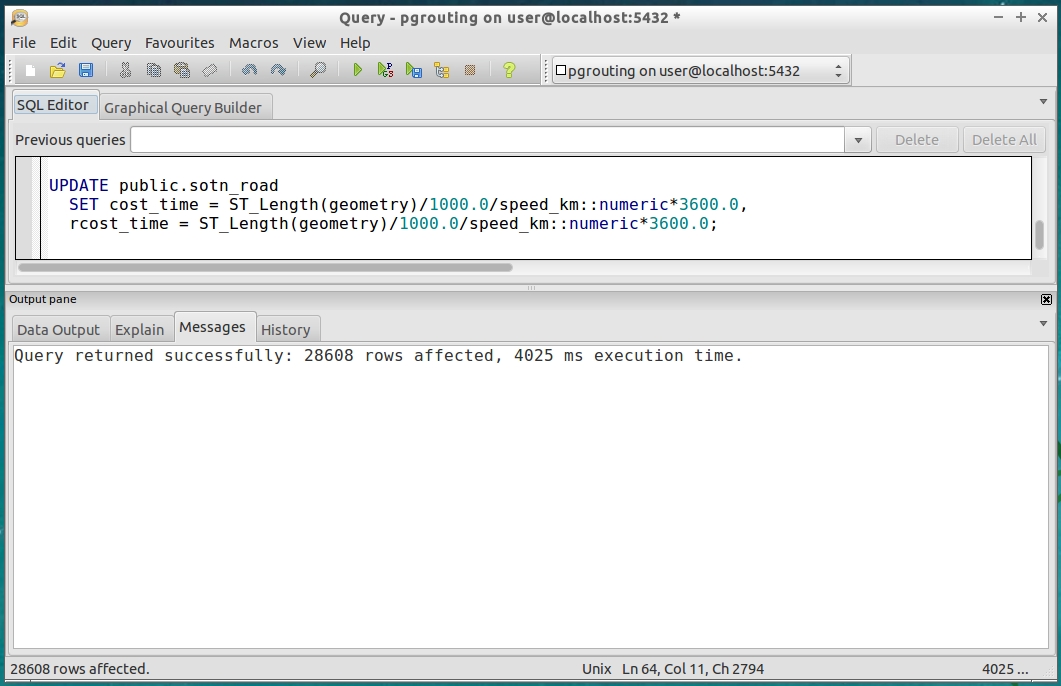
4.6 Then use the speed and length to calulate road link travel time.
UPDATE public.roadlink
  SET cost_time = ST_Length(geometry)/1000.0/speed_km::numeric*3600.0,
  rcost_time = ST_Length(geometry)/1000.0/speed_km::numeric*3600.0;
It’s worth noting here that OS Open Roads has been designed as a high level road network for quick and dirty routing and as such does not have the extra detail required for turn restrictions and one way streets. ITN and the new Highways layer have got the road routing information (RRI) detail.
Step 5: Building the network
Now that we have added all the fields and populated them with some reasonable values we can build our network topology. This will take about a minute.
SELECT public.pgr_createTopology('public.roadlink', 0.001, 'geometry', 'gid', 'source', 'target');
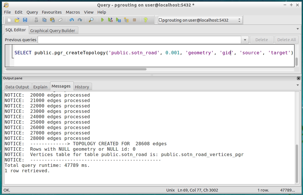
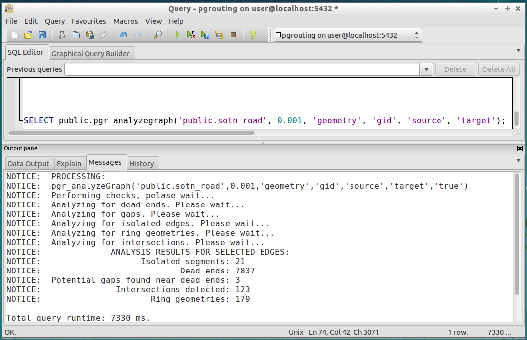
It is always a good idea to analyse your network graph as it will highlight potential errors. There will be some isolated segments, dead ends, potential gaps, intersections and ring geometries.
SELECT public.pgr_analyzegraph('public.roadlink', 0.001, 'geometry', 'gid', 'source', 'target');
Before we use the network it’s a good idea to clean up the table after all the additions and changes to it.
VACUUM ANALYZE VERBOSE public.roadlink;
Now we are ready to route!
Step 6: Routing in QGIS
Start or switch to QGIS.
Add the roadlink layer from PostGIS if not already loaded.
Add the PgRouting Layer plugin through Plugins > Install and Manage Plugins
You will need to go to Settings and check the experimental box and then back to the All tab to search for pgRouting. Check the box next to the plugin and click Install.
The plugin should appear in a docked panel in QGIS. If it doesn’t, right click on an empty space on the menu bar and check the box in the context menu to add it.
To configure the plugin we need to:
- set the database connection –
pgrouting - name the network table –
roadlink - set the unique identifier –
gid - set the source and target fields –
sourceandtarget - set the cost fields –
cost_lenandrcost_len(orcost_timeandrcost_time)
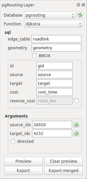
Once configured, we can set the routing function to djikstra and use the pickers to select the start and end points for our first route.
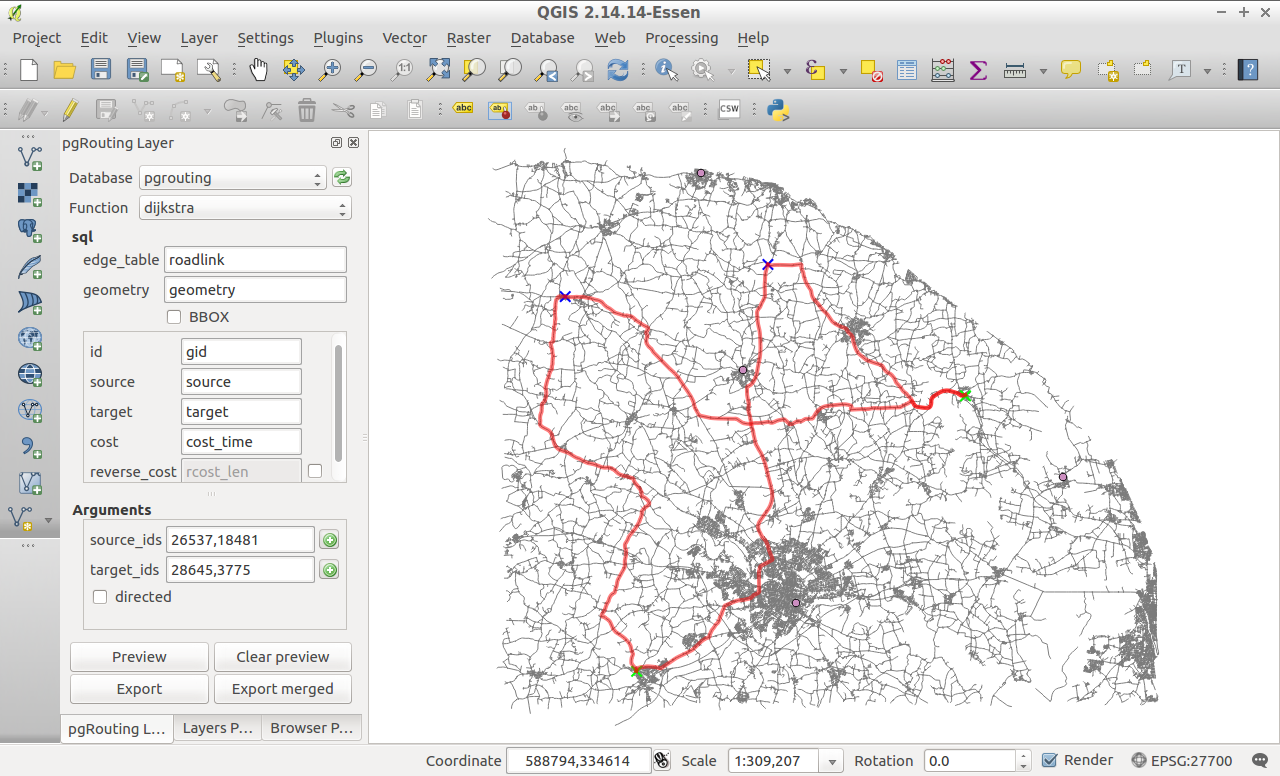
Try changing the cost fields from distance (cost_len / rcost_len) to time (cost_time / rcost_time) and see if the route changes.
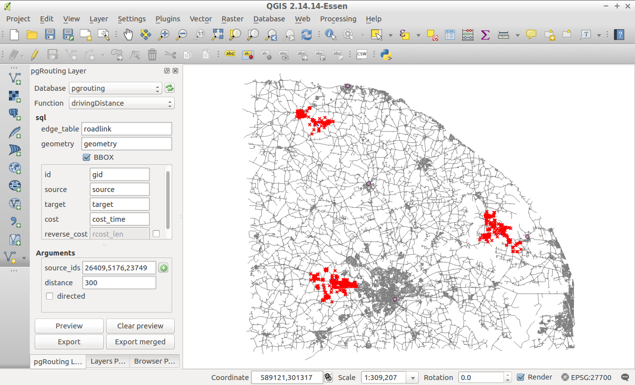
Select the driving distance function and pick a start node and then a distance (metres) or time (seconds) and see the rash of red nodes that indicate the nodes reachable within the specified cost.
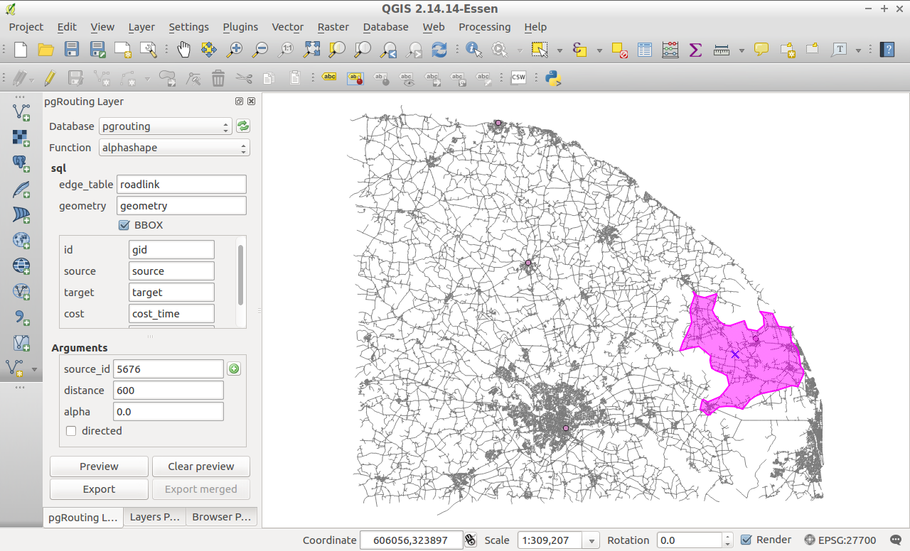
Select the alphashape function and use the same start node and cost set above and see the lovely pink result. The alphashape is like a shrink-wrapped convex hull around the set of points.
Step 7: Routing with SQL in PgAdminIII
Open or switch back to PgAdminIII.
Navigate to the pgrouting database and open a SQL editor window.
To calculate the shortest path between two points on the network we can use the Djikstra function like this:
SELECT seq, id1 AS node, id2 AS edge, cost FROM pgr_dijkstra('
SELECT gid AS id,
     source::integer,
     target::integer,
     cost_len::double precision AS cost
    FROM roadlink',
26920, 4232, false, false);
To try another function between the same start and end points we can use the A-star function. This uses the geographical information we added earlier (x1, y1, x2, y2) to prefer network links that are closest to the target of the shortest path search.
SELECT seq, id1 AS node, id2 AS edge, cost FROM pgr_astar('
SELECT gid AS id,
     source::integer,
     target::integer,
     cost_len::double precision AS cost,
     x1, y1, x2, y2
    FROM roadlink',
22661, 25892, false, false);
Driving distance is a useful function as a number of other functions hang off it including pgr_alphashape and pgr_pointsAsPolygon. The functions below show the links reachable within 2000m of the centre of Acle, Norfolk:
SELECT *
FROM pgr_drivingDistance(
        'SELECT gid AS id, source, target, cost_len AS cost FROM roadlink',
        24722, 2000
);
Within 5 minutes of the centre of Acle, Norfolk:
SELECT *
FROM pgr_drivingDistance(
        'SELECT gid AS id, source, target, cost_time AS cost FROM roadlink',
        24722, 300
);
The alphashape function is a bit more complex as it uses a number of PostGIS and pgRouting functions to generate the resulting polygon. Copy and paste the SQL below into your SQL window and run it.
We need to create a temporary node table first (should be about double the number of nodes in the network):
CREATE TEMPORARY TABLE node AS
SELECT id, ST_X(geometry) AS x, ST_Y(geometry) AS y, geometry
	FROM (
	    SELECT source AS id,
		ST_Startpoint(geometry) AS geometry
		FROM roadlink
	    UNION
	    SELECT target AS id,
		ST_Startpoint(geometry) AS geometry
		FROM roadlink
	) AS node;
Copy and paste this SQL to generate the alphashape for 10 minutes travel (600 seconds) from somewhere in Norfolk.
SELECT ST_SetSRID(ST_MakePolygon(ST_AddPoint(foo.openline, ST_StartPoint(foo.openline))),27700) AS geometry
	FROM (
	  SELECT ST_Makeline(points ORDER BY id) AS openline
	  FROM (
	    SELECT row_number() over() AS id, ST_MakePoint(x, y) AS points
	    FROM pgr_alphashape('
		SELECT *
		FROM node
		    JOIN
		    (SELECT * FROM pgr_drivingDistance(''
     			SELECT gid AS id,
     			source::int4 AS source,
     			target::int4 AS target,
     			cost_time::float8 AS cost,
     			rcost_time::float8 AS reverse_cost
     			FROM roadlink'',
     			13631,
     			600,
     			true,
     			true)) AS dd ON node.id = dd.id1'::text)
	  ) AS a
	) AS foo;
What the SQL above does is run the driving distance function which returns a set of records to the alphashape function. The alphashape function returns a table of XY rows describing the vertices of the alphashape polygon. These coordinates are converted to points and then lines and then, finally, a polygon. It is important to note that the alphashape code has no control over the order of the points so the output shapes may not be the same but will be similar.
Step 8: Adding some service locations
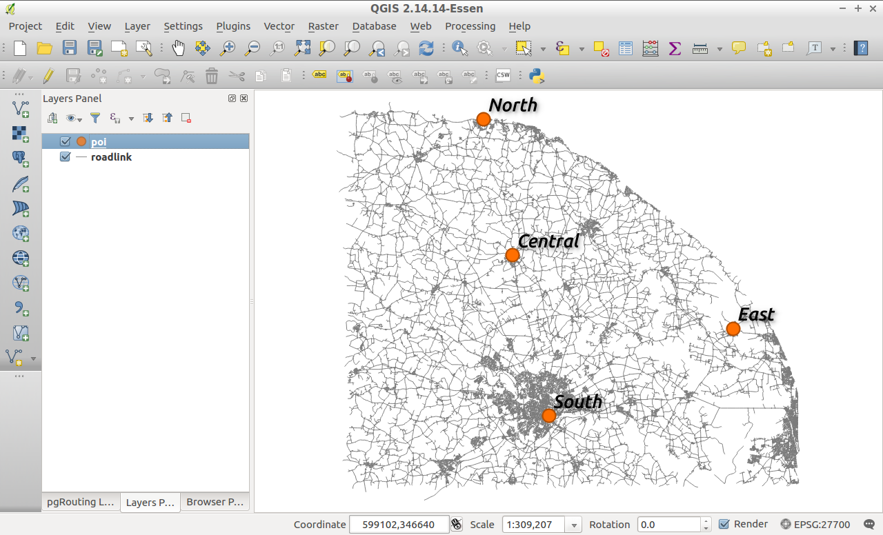
Add the poi.shp file to the QGIS canvas. You will see four dots on the map.
Open the Processing toolbox and find the PostGIS loading tool we used earlier. Open it and set it up to load the poi shapefile into the database. Make sure to set the coordinate system to EPSG:27700, the unique id field to gid and the geometry column to geometry. Uncheck promote to multipart.
Open or switch to PgAdminIII and connect to the pgRouting database. Open a SQL editor window.
Copy and paste the following SQL into the editor window:
ALTER TABLE public.poi
ADD COLUMN nearest_node integer;

CREATE TEMPORARY TABLE temp AS
   SELECT a.gid, b.id, min(a.dist)
   FROM
     (SELECT poi.gid,
             min(ST_distance(poi.geometry,  roadlink_vertices_pgr.the_geom)) AS dist
      FROM poi, roadlink_vertices_pgr
      GROUP BY poi.gid) AS a,
     (SELECT poi.gid, roadlink_vertices_pgr.id,
             ST_distance(poi.geometry, roadlink_vertices_pgr.the_geom) AS dist
   FROM poi, roadlink_vertices_pgr) AS b
   WHERE a.dist = b. dist
   AND a.gid = b.gid
   GROUP BY a.gid, b.id;

UPDATE poi
SET nearest_node =
   (SELECT id
    FROM temp
    WHERE temp.gid = poi.gid);
This SQL assigns each of the points in the poi layer a node ID from the roadlink network. We’ll use this information to create a function to compute alphashapes for each of the points of interest.
Step 9: Creating an alphashape function
I expect we’ll be running short of time round about now so again this is a copy and paste exercise and I’ll explain what this function does below. Hopefully the comments will help.
CREATE OR REPLACE FUNCTION public.make_isochronesx(v_input text, v_cost integer)
  RETURNS integer AS
$BODY$
DECLARE
	cur_src refcursor;    --set some variables
	v_nn integer;
	v_geom geometry;
	v_tbl varchar(200);
	v_sql varchar(1000);
BEGIN
	RAISE NOTICE 'Dropping isochrone table...';
	-- Drop the table being created if it exists
	v_sql:='DROP TABLE IF EXISTS public.'||v_input||'_iso_'||v_cost;
	EXECUTE v_sql;
	RAISE NOTICE 'Creating isochrone table...';
	-- Create the table to hold the data if it doesn't exist
	v_sql:='CREATE TABLE IF NOT EXISTS public.'||v_input||'_iso_'||v_cost||'
		( id serial NOT NULL,
		  node_id integer,
		  geometry geometry(Polygon,27700),
		  CONSTRAINT '||v_input||'_iso_'||v_cost||'_pkey PRIMARY KEY (id)
		);
		CREATE INDEX '||v_input||'_iso_'||v_cost||'_geometry
		  ON public.'||v_input||'_iso_'||v_cost||'
		  USING gist
		  (geometry);';
	EXECUTE v_sql;
	RAISE NOTICE 'Creating temporary node table...';
	-- Drop then recreate temporary node table from roadlinks used in generating isochrones
	DROP TABLE IF EXISTS node;
	CREATE TEMPORARY TABLE node AS
	    SELECT id,
		ST_X(geometry) AS x,
		ST_Y(geometry) AS y,
		geometry
		FROM (
		    SELECT source AS id,
			ST_Startpoint(geometry) AS geometry
			FROM roadlink
		    UNION
		    SELECT target AS id,
			ST_Startpoint(geometry) AS geometry
			FROM roadlink
		) AS node;
	RAISE NOTICE 'Calculating isochrones...';
	-- Loop through the input features, creating an isochrone for each one, and insert into the output table
	OPEN cur_src FOR EXECUTE format('SELECT nearest_node FROM '||v_input);
	LOOP
	FETCH cur_src INTO v_nn;
	EXIT WHEN NOT FOUND;
	SELECT ST_SetSRID(ST_MakePolygon(ST_AddPoint(foo.openline, ST_StartPoint(foo.openline))),27700) AS geometry
	FROM (
	  SELECT ST_Makeline(points ORDER BY id) AS openline
	  FROM (
	    SELECT row_number() over() AS id, ST_MakePoint(x, y) AS points
	    FROM pgr_alphashape('
		SELECT *
		FROM node
		    JOIN
		    (SELECT * FROM pgr_drivingDistance(''
			SELECT gid AS id,
			source::int4 AS source,
			target::int4 AS target,
			cost_time::float8 AS cost,
			rcost_time::float8 AS reverse_cost
			FROM roadlink'',
			'||v_nn||',
			'||v_cost||',
			true,
			true)) AS dd ON node.id = dd.id1'::text)
	  ) AS a
	) AS foo INTO v_geom;
	-- Set the table name
	v_tbl:='public.'||v_input||'_iso_'||v_cost;
	-- Insert the isochrone geometries into the table
	EXECUTE format('INSERT INTO %s(node_id,geometry) VALUES ($1,$2)',v_tbl)
		USING v_nn, v_geom;
	END LOOP;
	RETURN 1;
	CLOSE cur_src;
END;
$BODY$
  LANGUAGE plpgsql VOLATILE
  COST 100;
Execute the SQL by pressing F5 or the RUN button. It should say that the query returned successfully with no result in xxx ms. Now we have a new function in the database that we can use to generate some alphashapes or isochrones around our points of interest layer.
In a nutshell then: the function creates a new table to hold the alphashape polygons. It drops and creates a temporary node table. It uses the node table to generate an alphashape for each input shape based on the cost given to the function at rumtime. These shapes are inserted into the polygon table. The function stops when all input features have been processed.
To execute the function we need the name of our POI table – poi – and a time interval. We’ll run the function a couple of times to generate multiple isochrones so 300, 600 and 900 should do.
SELECT public.make_isochronesx('poi', 300);

SELECT public.make_isochronesx('poi', 600);

SELECT public.make_isochronesx('poi', 900);
Back in QGIS, refresh your pgrouting database connection and you’ll see the new tables. Add them to the canvas and you’ll get something like this:
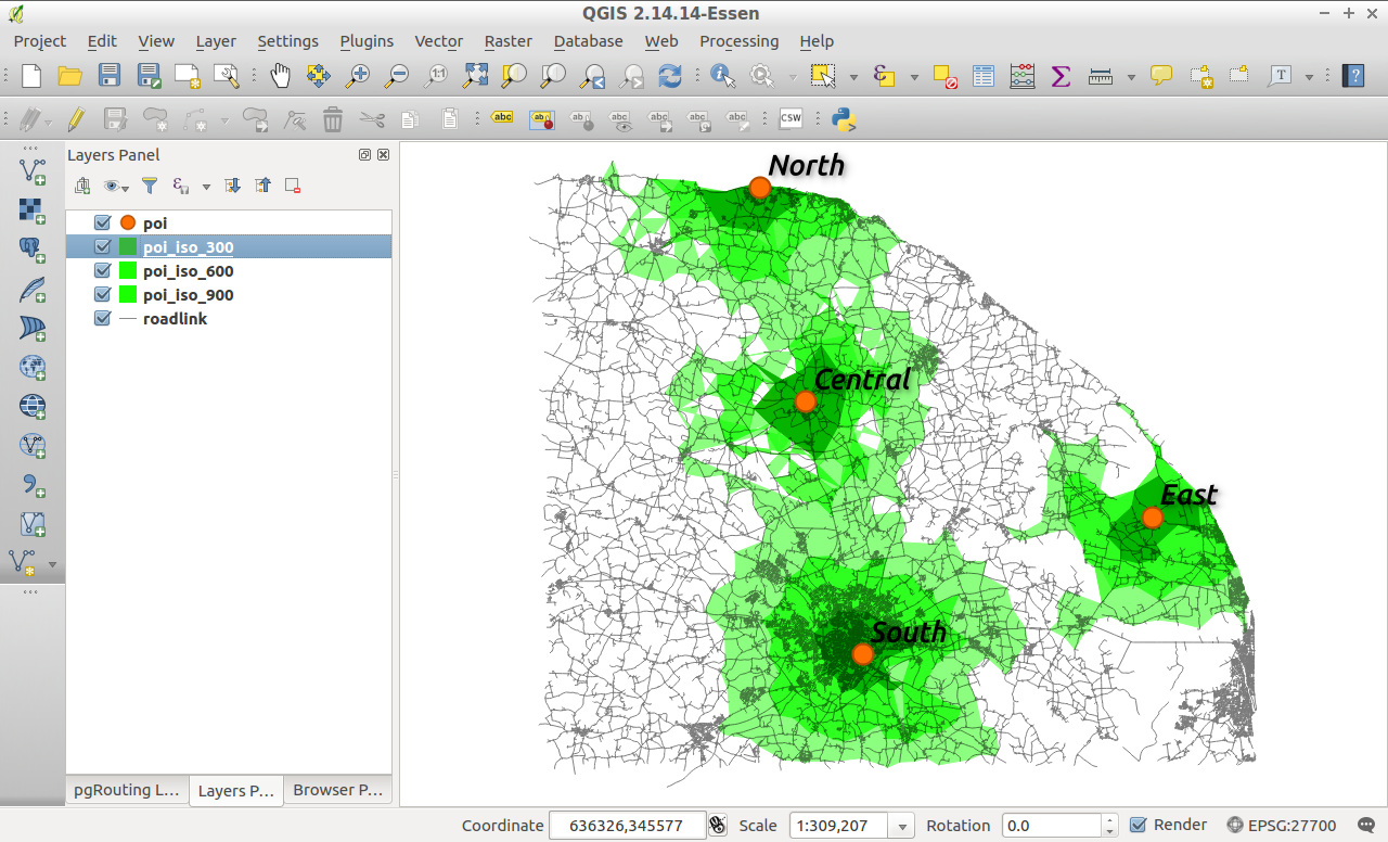
5, 10 and 15 minute isochrones
References and supporting documentation